Data Flow Inside a Neural Network Model

Inside a Neural Network Model, when we pass in a value it should some other value.

Let’s inspect an example model

import torch
import torch.nn as nn

class NeuralNetwork(nn.Module):
    def __init__(self):
        super(NeuralNetwork, self).__init__()
        self.input_layer = nn.Linear(1, 1)

    def forward(self, x):
        x = self.input_layer(x)
        return x

Here, we have a simple neural network model with a single input and output layer. The input layer has a single node and the output layer has a single node.

When we pass a value to this model, it will multiply the input value with a weight and add a bias to it. This is the basic operation of a linear layer.

The output of this model is calculated as follows,

model = NeuralNetwork()
input_value = torch.tensor([1.0])

output = model(input_value)
for name, param in model.named_parameters():
    print(name, param.item())
print(output.item())

When running this code, we will get the output as follows,

linear.weight 0.35672545433044434
linear.bias -0.23311853408813477
0.12360692024230957

The weight and bias are randomly initialized values. The output is calculated as output = input_value * weight + bias.

This is the basic operation of a neural network model. It takes an input value, multiplies it with a weight, adds a bias to it, and returns the output.

here, the operation will be like this,

output = model.linear.weight.item() * input_value + model.linear.bias.item()

Note: item() works only for scalar values, for tensors use param.tolist() instead.

similarly, we can have a different model with more inputs

import torch
import torch.nn as nn
import torch.optim as optim

# simple linear model
class LinearRegression(nn.Module):
    def __init__(self):
        super(LinearRegression, self).__init__()
        self.linear = nn.Linear(2, 1)

    def forward(self, x):
        return self.linear(x)

model = LinearRegression()

x = torch.tensor([1.0, 2.0], requires_grad=True)
y = model(x)
for name, value in model.named_parameters():
    print(name, value.tolist())
print(y.tolist())

which would output something like

linear.weight [[0.611233651638031, 0.3145529627799988]]
linear.bias [-0.34737372398376465]
[0.8929657936096191]

the calculation would be like, output = input_value[0] * weight[0] + input_value[1] * weight[1] + bias

Adjustments during Training

During training, the weights and biases of the model are adjusted to minimize the loss. The loss is calculated based on the difference between the predicted output and the actual output.

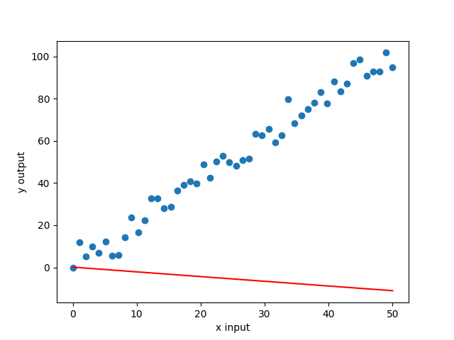
Let’s plot the real vs predicted graph for a simple linear regression model.

import matplotlib.pyplot as plt
import torch
import torch.nn as nn
import torch.optim as optim


# simple linear model
class LinearRegression(nn.Module):
    def __init__(self):
        super(LinearRegression, self).__init__()
        self.linear = nn.Linear(1, 1)

    def forward(self, x):
        return self.linear(x)

model = LinearRegression()

simple_list = torch.linspace(0, 50, 50).view(-1, 1)
noise = torch.randn(simple_list.shape) * 5

# Define a simple linear function with some noise
desired_data = 2 * simple_list + 1 + noise

# Define a predicted 
predicted_data = model(simple_list)

plt.scatter(simple_list, desired_function)
plt.plot(simple_list, predicted_function.data, 'r')
plt.ylabel('y output')
plt.xlabel('x input')
plt.show()
plt.savefig('initial_state.png')

we get a graph something like this, ( depends on weight and bias values )

real vs predicted

The goal of training is to move the red line closer to the blue dots. This is done by adjusting the weights and biases of the model.

a loss function will be used to calculate the difference between the predicted and actual output and an optimizer will be used to adjust the weights and biases of the model to minimize the loss.

criterion = nn.MSELoss()
optimizer = optim.SGD(model.parameters(), lr=0.0001)

# Training loop
epochs = 100
losses = []
for i in range(epochs):
    i += 1
    # Predict the output
    predicted_function = model(simple_list)
    # Calculate the loss
    loss = criterion(predicted_function, desired_function)
    losses.append(loss.item()) # to plot the loss
    # Zero the gradients
    optimizer.zero_grad()
    # Backward pass - Calculate the gradients for the weights and biases
    loss.backward()
    # Update the weights and biases based on the calculated gradients
    optimizer.step()

    if i % 10 == 0:
        print(f'epoch {i} loss: {loss.item()} weight: {model.linear.weight.item()} bias: {model.linear.bias.item()}')

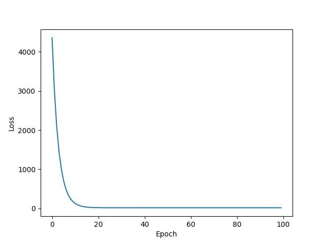
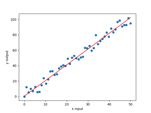
finally when we can plot the loss and the predicted graph

# Get the final prediction
predicted_function = model(simple_list)

plt.plot(range(epochs), losses)
plt.ylabel('Loss')
plt.xlabel('Epoch')
plt.show()

plt.scatter(simple_list, desired_function)
plt.plot(simple_list, predicted_function.data, 'r')
plt.ylabel('y output')
plt.xlabel('x input')
plt.show()

we get a graph something like this,

Loss graph

loss graph

Final Prediction

final prediction

Summary

A neural network model takes an input value, multiplies it with a weight, adds a bias to it, and returns the output.
The network starts with a random initialization of weights and biases.
During training, the weights and biases are adjusted to minimize the loss.
The loss is calculated based on the difference between the predicted output and the actual output.

Data Flow Inside a Neural Network Model#

Adjustments during Training#

Data Flow Inside a Neural Network Model

Adjustments during Training